Notes on: Rabiner, L. R. (1990): A tutorial on hidden markov models and selected applications in speech recognition
@article{Rabiner_tutor_HMM,
  author    = {Rabiner, Lawrence R.},
  title     = {A Tutorial on Hidden Markov Models and Selected Applications in Speech Recognition},
  journal   = {Readings in Speech Recognition},
  pages     = {267–296},
  year      = {1990},
  doi       = {10.1016/b978-0-08-051584-7.50027-9},
  url       = {http://dx.doi.org/10.1016/b978-0-08-051584-7.50027-9},
  isbn      = {http://id.crossref.org/isbn/9781558601246},
  publisher = {Elsevier BV},
}
Although initially introduced and studied in the late 1960s and early 1970s, statistical methods of Markov source or hidden Markov modeling have become increasingly popular in the last several years. There are two strong reasons why this has occurred. First the models are very rich in mathematical structure and hence can form the theoretical basis for use in a wide range of applications. Second the models, when applied properly, work very well in practice for several important applications. In this paper we attempt to carefully and methodically review the theoretical aspects of this type of statistical modeling and show how they have been applied to selected problems in machine recognition of speech.
INTRODUCTION
Real-world processes generally produce observable outputs which can be characterized as signals. The signals can be discrete in nature (e.g., characters from a finite alphabet, quantized vectors from a codebook, etc.), or continuous in nature (e.g., speech samples, temperature measurements, music, etc.). The signal source can be stationary (i.e., its statistical properties do not vary with time), or nonstationary (i.e., the signal properties vary over time). The signals can be pure (i.e., coming strictly from a single source), or can be corrupted from other signal sources (e.g., noise) or by transmission distortions, reverberation, etc.
A problem of fundamental interest is characterizing such real-world signals in terms of signal models. There are several reasons why one is interested in applying signal models. First of all, a signal model can provide the basis for a theoretical description of a signal processing system which can be used to process the signal so as to provide a desired output. For example if we are interested in enhancing a speech signal corrupted by noise and transmission distortion, we can use the signal model to design a system which will optimally remove the noise and undo the transmission distortion. A second reason why signal models are important is that they are potentially capable of letting us learn a great deal about the signal source (i.e., the real-world process which produced the signal) without having to have the source available. This property is especially important when the cost of getting signals from the actual source is high. In this case, with a good signal model, we can simulate the source and learn as much as possible via simulations. Finally, the most important reason why signal models are important is that they often work extremely well in practice, and enable us to realize important practical systems-e.g., prediction systems, recognition systems, identification systems, etc., in a very efficient manner.
These are several possible choices for what type of signal model is used for characterizing the properties of a given signal. Broadly one can dichotomize the types of signal models into the class of deterministic models, and the class of statistical models. Deterministic models generally exploit some known specific properties of the signal, e.g., that the signal is a sine wave, or a sum of exponentials, etc. In these cases, specification of the signal model is generally straightforward; all that is required is to determine (estimate) values of the parameters of the signal model (e.g., amplitude, frequency, phase of a sine wave, amplitudes and rates of exponentials, etc.). The second broad class of signal models is the set of statistical models in which one tries to characterize only the statistical properties of the signal. Examples of such statistical models include Gaussian processes, Poisson processes, Markov processes, and hidden Markov processes, among others. The underlying assumption of the statistical model is that the signal can be well characterized as a parametric random process, and that the parameters of the stochastic process can be determined (estimated) in a precise, well-defined manner.
For the applications of interest, namely speech processing, both deterministic and stochastic signal models have had good success. In this paper we will concern ourselves strictly with one type of stochastic signal model, namely the hidden Markov model (HMM). (These models are referred to as Markov sources or probabilistic functions of Markov chains in the communications literature.) We will first review the theory of Markov chains and then extend the ideas to the class of hidden Markov models using several simple examples. We will then focus our attention on the three fundamental problems 1 for HMM design, namely: the evaluation of the probability (or likelihood) of a sequence of observations given a specific HMM; the determination of a best sequence of model states; and the adjustment of model parameters so as to best account for the observed signal. We will show that once these three fundamental problems are solved, we can apply HMMs to selected problems in speech recognition.
Neither the theory of hidden Markov models nor its applications to speech recognition is new. The basic theory was published in a series of classic papers by Baum and his colleagues [Ref1], [Ref2], [Ref3], [Ref4], [Ref5] in the late 1960s and early 1970s and was implemented for speech processing applications by Baker [Ref6] at CMU, and by Jelinek and his colleagues at IBM [Ref7], [Ref8], [Ref9], [Ref10], [Ref11], [Ref12], [Ref13] in the 1970s. However, widespread understanding and application of the theory of HMMs to speech processing has occurred only within the past several years. There are several reasons why this has been the case. First, the basic theory of hidden Markov models was published in mathematical journals which were not generally read by engineers working on problems in speech processing. The second reason was that the original applications of the theory to speech processing did not provide sufficient tutorial material for most readers to understand the theory and to be able to apply it to their own research. As a result, several tutorial papers were written which provided a sufficient level of detail for a number of research labs to begin work using HMMs in individual speech processing applications [Ref14], [Ref15], [Ref16], [Ref17], [Ref18], [Ref19]. This tutorial is intended to provide an overview of the basic theory of HMMs (as originated by Baum and his colleagues), provide practical details on methods of implementation of the theory, and describe a couple of selected applications of the theory to distinct problems in speech recognition. The paper combines results from a number of original sources and hopefully provides a single source for acquiring the background required to pursue further this fascinating area of research.
The organization of this paper is as follows. In Section II we review the theory of discrete Markov chains and show how the concept of hidden states, where the observation is a probabilistic function of the state, can be used effectively. We illustrate the theory with two simple examples, namely coin-tossing, and the classic balls-in-urns system. In Section III we discuss the three fundamental problems of HMMs, and give several practical techniques for solving these problems. In Section IV we discuss the various types of HMMs that have been studied including ergodic as well as left-right models. In this section we also discuss the various model features including the form of the observation density function, the state duration density, and the optimization criterion for choosing optimal HMM parameter values. In Section V we discuss the issues that arise in implementing HMMs including the topics of scaling, initial parameter estimates, model size, model form, missing data, and multiple observation sequences. In Section VI we describe an isolated word speech recognizer, implemented with HMM ideas, and show how it performs as compared to alternative implementations. In Section VII we extend the ideas presented in Section VI to the problem of recognizing a string of spoken words based on concatenating individual HMMs of each word in the vocabulary. In Section VIII we briefly outline how the ideas of HMM have been applied to a large vocabulary speech recognizer, and in Section IX we summarize the ideas discussed throughout the paper.
DISCRETE MARKOV PROCESSES 2
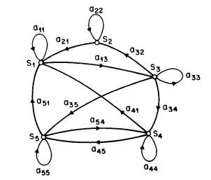
图 1 A Markov chain with 5 states (labeled \(S_1\) to \(S_5\)) with selected state transitions.
Consider a system which may be described at any time as being in one of a set of \(N\) distinct states, \(S_1, S_2, \ldots, S_N\), as illustrated in 图 1 (where \(N = 5\) for simplicity). At regularly spaced discrete times, the system undergoes a change of state (possibly back to the same state) according to a set of probabilities associated with the state. We denote the time instants associated with state changes as \(t = 1, 2, \ldots\) , and we denote the actual state at time \(t\) as \(q_t\). A full probabilistic description of the above system would, in general, require specification of the current state (at time \(t\)), as well as all the predecessor states. For the special case of a discrete, first order, Markov chain, this probabilistic description is truncated to just the current and the predecessor state, i.e.,
Further more we only consider those processes in which the right-hand side of (1) is independent of time, thereby leading to the set of state transition probabilities \(a_{ij}\) of the form
with the state transition coefficients having the properties
since they obey standard stochastic constraints.
The above stochastic process could be called an observable Markov model since the output of the process is the set of states at each instant of time, where each state corresponds to a physical (observable) event. To set ideas, consider a simple 3-state Markov model of the weather. We assume that once a day (e.g., at noon), the weather is observed as being one of the following:
State 1: rain or (snow)
State 2: cloudy
State 3: sunny
We postulate that the weather on day \(t\) is characterized by a single one of the three states above, and that the matrix \(A\) of state transition probabilities is
Given that the weather on day 1 (\(t = 1\)) is sunny (state 3), we can ask the question: What is the probability (according to the model) that the weather for the next 7 days will be “sun-sun-rain-rain-sun-cloudy-sun”? Stated more formally, we define the observation sequence \(O\) as \(O = \{S_3, S_3, S_3, S_1, S_1, S_3, S_2, S_3\}\) corresponding to \(t = 1, 2, \ldots, 8,\) and we wish to determine the probability of \(O\) , given the model. This probability can be expressed (and evaluated) as
where we use the notation
to denote the initial state probabilities.
Another interesting question we can ask (and answer using the model) is: Given that the model is in a known state, what is the probability it stays in that state for exactly \(d\) days? This probability can be evaluated as the probability of the observation sequence
given the model, which is
The quantity \(p_i(d)\) is the (discrete) probability density function of duration \(d\) in state \(i\) . This exponential duration density is characteristic of the state duration in a Markov chain. Based on \(p_i(d)\) , we can readily calculate the expected number of observations (duration) in a state, conditioned on starting in that state as
Thus the expected number of consecutive days of sunny weather, according to the model, is \(1/0.2 = 5\) ; for cloudy it is \(2.5\) ; for rain it is \(1.67\) .
Extension to Hidden Markov Models
So far we have considered Markov models in which each state corresponded to an observable (physical) event. This model is too restrictive to be applicable to many problems of interest. In this section we extend the concept of Markov models to include the case where the observation is a probabilistic function of the state-i.e., the resulting model (which is called a hidden Markov model) is a doubly embedded stochastic process with an underlying stochastic process that is not observable (it is hidden), but can only be observed through another set of stochastic processes that produce the sequence of observations. To fix ideas, consider the following model of some simple coin tossing experiments.
Coin Toss Models: Assume the following scenario. You are in a room with a barrier (e.g., a curtain) through which you cannot see what is happening. On the other side of the barrier is another person who is performing a coin (or multiple coin) tossing experiment. The other person will not tell you anything about what he is doing exactly; he will only tell you the result of each coin flip. Thus a sequence of hidden coin tossing experiments is performed, with the observation sequence consisting of a series of heads and tails; e.g., a typical observation sequence would be
where \(\mathscr{H}\) stands for heads and \(\mathscr{T}\) stands for tails.
Given the above scenario, the problem of interest is how do we build an HMM to explain (model) the observed sequence of heads and tails. The first problem one faces is deciding what the states in the model correspond to, and then deciding how many states should be in the model. One possible choice would be to assume that only a single biased coin was being tossed. In this case we could model the situation with a 2-state model where each state corresponds to a side of the coin (i.e., heads or tails). This model is depicted in 图 2 (a) 3. In this case the Markov model is observable, and the only issue for complete specification of the model would be to decide on the best value for the bias (i.e., the probability of, say, heads). Interestingly, an equivalent HMM to that of 图 2 (a) would be a degenerate 1-state model, where the state corresponds to the single biased coin, and the unknown parameter is the bias of the coin.
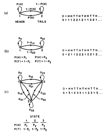
图 2 Three possible Markov models which can account for the results of hidden coin tossing experiments. (a) 1-coin model. (b) 2-coins model. (c) 3-coins model.
A second form of HMM for explaining the observed sequence of coin toss outcome is given in 图 2 (b). In this case there are 2 states in the model and each state corresponds to a different, biased, coin being tossed. Each state is characterized by a probability distribution of heads and tails, and transitions between states are characterized by a state transition matrix. The physical mechanism which accounts for how state transitions are selected could itself be a set of independent coin tosses, or some other probabilistic event.
A third form of HMM for explaining the observed sequence of coin toss outcomes is given in 图 2 (c). This model corresponds to using 3 biased coins, and choosing from among the three, based on some probabilistic event.
Given the choice among the three models shown in 图 2 for explaining the observed sequence of heads and tails, a natural question would be which model best matches the actual observations. It should be clear that the simple 1-coin model of 图 2 (a) has only 1 unknown parameter; the 2-coin model of 图 2 (b) has 4 unknown parameters; and the 3-coin model of 图 2 (c) has 9 unknown parameters. Thus, with the greater degrees of freedom, the larger HMMs would seem to inherently be more capable of modeling a series of coin tossing experiments than would equivalently smaller models. Although this is theoretically true, we will see later in this paper that practical considerations impose some strong limitations on the size of models that we can consider. Furthermore, it might just be the case that only a single coin is being tossed. Then using the 3-coin model of 图 2 (c) would be inappropriate, since the actual physical event would not correspond to the model being used-i.e., we would be using an underspecified system.
The Urn and Ball Mode 4: To extend the ideas of the HMM to a somewhat more complicated situation, consider the urn and ball system of 图 3 . We assume that there are \(N\) (large) glass urns in a room. Within each urn there are a large number of colored balls. We assume there are \(M\) distinct colors of the balls. The physical process for obtaining observations is as follows. A genie is in the room, and according to some random process, he (or she) chooses an initial urn. From this urn, a ball is chosen at random, and its color is recorded as the observation. The ball is then replaced in the urn from which it was selected. A new urn is then selected according to the random selection process associated with the current urn, and the ball selection process is repeated. This entire process generates a finite observation sequence of colors, which we would like to model as the observable output of an HMM.
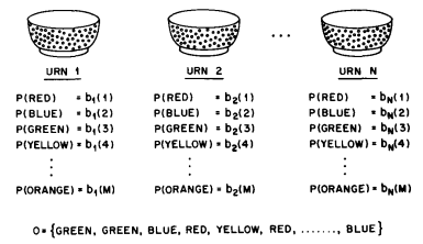
图 3 An \(N\text{-state}\) urn and ball model which illustrates the general case of a discrete symbol HMM.
It should be obvious that the simplest HMM that corresponds to the urn and ball process is one in which each state corresponds to a specific urn, and for which a (ball) color probability is defined for each state. The choice of urns is dictated by the state transition matrix of the HMM.
Elements of an HMM
The above examples give us a pretty good idea of what an HMM is and how it can be applied to some simple scenarios. We now formally define the elements of an HMM, and explain how the model generates observation sequences.
An HMM is characterized by the following:
\(N\), the number of states in the model. Although the states are hidden, for many practical applications there is often some physical significance attached to the states or to sets of states of the model. Hence, in the coin tossing experiments, each state corresponded to a distinct biased coin. In the urn and ball model, the states corresponded to the urns. Generally the states are interconnected in such a way that any state can be reached from any other state (e.g., an ergodic model); however, we will see later in this paper that other possible interconnections of states are often of interest. We denote the individual states as \(S = \{S_1, S_2, \ldots, S_N\}\), and the state at time \(t\) as \(q_t\).
\(M\), the number of distinct observation symbols per state, i.e., the discrete alphabet size. The observation symbols correspond to the physical output of the system being modeled. For the coin toss experiments the observation symbols were simply heads or tails; for the ball and urn model they were the colors of the balls selected from the urns. We denote the individual symbols as \(V = \{v_1, v_2, \ldots, v_M\}\).
The state transition probability distribution \(A = \{a_{ij}\}\) where
(7)¶\[a_{ij} = P[q_{t+1} = S_j \mid q_t = S_i], \quad 1 \leq i, j \leq N.\]For the special case where any state can reach any other state in a single step, we have \(a_{ij} > 0\) for all \(i, j\) . For other types of HMMs, we would have \(a_{ij} = 0\) for one or more \((i,j)\) pairs.
The observation symbol probability distribution in state \(j\), \(B = \{b_j(k)\}\), where
(8)¶\[b_j(k) = P[v_k \text{ at } t \mid q_t = S_j], \quad 1 \leq j \leq N, \quad 1 \leq k \leq M.\]The initial state distribution \(\pi = \{\pi_i\}\) where
(9)¶\[\pi_i = P[q_1 = S_i], \quad 1 \leq i \leq N.\]
Given appropriate values of \(N, M, A, B\), and \(\pi\), the HMM can be used as a generator to give an observation sequence
(where each observation \(O_t\) is one of the symbols from \(V\), and \(T\) is the number of observations in the sequence) as follows:
Choose an initial state \(q_1 = S_i\) according to the initial state distribution \(\pi\).
Set \(t = 1\).
Choose \(O_t = v_k\) according to the symbol probability distribution in state \(S_i\), i.e., \(b_i(k)\).
Transit to a new state \(q_{t+1} = S_j\) according to the state transition probability distribution for state \(S_i\), i.e., \(a_{ij}\).
Set \(t = t + 1\); return to step 3 if \(t < T\); otherwise terminate the procedure.
The above procedure can be used as both a generator of observations, and as a model for how a given observation sequence was generated by an appropriate HMM.
It can be seen from the above discussion that a complete specification of an HMM requires specification of two model parameters (\(N\) and \(M\)), specification of observation symbols, and the specification of the three probability measures \(A, B\), and \(\pi\) . For convenience, we use the compact notation
to indicate the complete parameter set of the model.
The Three Basic Problems for HMMs 5
Given the form of HMM of the previous section, there are three basic problems of interest that must be solved for the model to be useful in real-world applications. These problems are the following:
Problem 1: Given the observation sequence \(\mathcal{O} = O_1 O_2 \cdots O_T\), and a model \(\lambda = (A, B, \pi)\), how do we efficiently compute \(P(\mathcal{O} \mid \lambda)\), the probability of the observation sequence, given the model?
Problem 2: Given the observation sequence \(\mathcal{O} = O_1 O_2 \cdots O_T\), and the model \(\lambda\), how do we choose a corresponding state sequence \(Q = q_1 q_2 \cdots q_T\) which is optimal in some meaningful sense (i.e., best “explains” the observations?)
Problem 3: How do we adjust the model parameters \(\lambda = (A, B, \pi)\) to maximize \(P(\mathcal{O} \mid \lambda)\)?
Problem 1 is the evaluation problem, namely given a model and a sequence of observations, how do we compute the probability that the observed sequence was produced by the model. We can also view the problem as one of scoring how well a given model matches a given observation sequence. The latter viewpoint is extremely useful. For example, if we consider the case in which we are trying to choose among several competing models, the solution to Problem 1 allows us to choose the model which best matches the observations.
Problem 2 is the one in which we attempt to uncover the hidden part of the model, i.e., to find the “correct” state sequence. It should be clear that for all but the case of degenerate models, there is no “correct” state sequence to be found. Hence for practical situations, we usually use an optimality criterion to solve this problem as best as possible. Unfortunately, as we will see, there are several reasonable optimality criteria that can be imposed, and hence the choice of criterion is a strong function of the intended use for the uncovered state sequence. Typical uses might be to learn about the structure of the model, to find optimal state sequences for continuous speech recognition, or to get average statistics of individual states, etc.
Problem 3 is the one in which we attempt to optimize the model parameters so as to best describe how a given observation sequence comes about. The observation sequence used to adjust the model parameters is called a training sequence since it is used to “train” the HMM. The training problem is the crucial one for most applications of HMMs, since it allows us to optimally adapt model parameters to observed training data-i.e., to create best models for real phenomena.
To fix ideas, consider the following simple isolated word speech recognizer. For each word of a \(W\) word vocabulary, we want to design a separate \(N\)-state HMM. We represent the speech signal of a given word as a time sequence of coded spectral vectors. We assume that the coding is done using a spectral codebook with \(M\) unique spectral vectors; hence each observation is the index of the spectral vector closest (in some spectral sense) to the original speech signal. Thus, for each vocabulary word, we have a training sequence consisting of a number of repetitions of sequences of codebook indices of the word (by one or more talkers). The first task is to build individual word models. This task is done by using the solution to Problem 3 to optimally estimate model parameters for each word model. To develop an understanding of the physical meaning of the model states, we use the solution to Problem 2 to segment each of the word training sequences into states, and then study the properties of the spectral vectors that lead to the observations occurring in each state. The goal here would be to make refinements on the model (e.g., more states, different codebook size, etc.) so as to improve its capability of modeling the spoken word sequences. Finally, once the set of \(W\) HMMs has been designed and optimized and thoroughly studied, recognition of an unknown word is performed using the solution to Problem 1 to score each word model based upon the given test observation sequence, and select the word whose model score is highest (i.e., the highest likelihood).
In the next section we present formal mathematical solutions to each of the three fundamental problems for HMMs. We shall see that the three problems are linked together tightly under our probabilistic framework.
SOLUTIONS TO THE THREE BASIC PROBLEMS OF HMMs
Solution to Problem 1
We wish to calculate the probability of the observation sequence, \(\mathcal{O} = O_1 O_2 \cdots O_T\), given the model \(\lambda\), i.e., \(P(\mathcal{O} \mid \lambda)\). The most straightforward way of doing this is through enumerating every possible state sequence of length \(T\) (the number of observations). Consider one such fixed state sequence
where \(q_1\) is the initial state. The probability of the observation sequence \(\mathcal{O}\) for the state sequence of (12) is
where we have assumed statistical indepencence of observations. Thus we get
The probability of such a state sequence \(Q\) can be written as
The joint probability of \(\mathcal{O}\) and \(Q\), i.e., the probability that \(\mathcal{O}\) and \(Q\) occur simultaneously, is simply the product of the above two terms, i.e.,
The probability of \(\mathcal{O}\) (given the model) is obtained by summing this joint probability over all possible state sequences \(Q\) giving
The interpretation of the computation in the above equation is the following. Initially (at time \(t = 1\)) we are in state \(q_1\) with probability \(\pi_{q_1}\), and generate the symbol \(O_1\) (in this state) with probability \(b_{q_1}(O_1)\). The clock changes from time \(t\) to \(t+1\) (\(t = 2\)) and we make a transition to state \(q_2\) from state \(q_1\) with probability \(a_{q_1 q_2}\), and generate symbol \(O_2\) with probability \(b_{q_2}(O_2)\). This process continues in this manner until we make the list transition (at time \(T\)) from state \(q_{T-1}\) to state \(q_T\) with probability \(a_{q_{T-1} q_T}\) and generate symbol \(O_T\) with probability \(b_{q_T}(O_T)\).
A little thought should convince the reader that the calculation of \(P(\mathcal{O} \mid \lambda)\), according to its direct definition (17) involves on the order of \(2 T \cdot N^T\) calculations, since at every \(t = 1, 2, \ldots, T\), there are \(N\) possible states which can be reached (i.e., there are \(N^T\) possible state sequences), and for each such state sequence about \(2T\) calculations are required for each term in the sum of (17). (To be precise, we need \((2T-1)N^T\) multiplications, and \(N^T-1\) additions.) This calculation is computationally unfeasible, even for small values of \(N\) and \(T\); e.g., for \(N = 5\) (states), \(T = 100\) (observations), there are on the order of \(2 \cdot 100 \cdot 5^{100} \approx 10^{72}\) computations! Clearly a more efficient procedure is required to solve Problem 1. Fortunately such a procedure exists and is called the forward-backward procedure.
The Forward-Backward Procedure 6 [Ref2], [Ref3]: Consider the forward variable \(\alpha_t(i)\) defined as
i.e., the probability of the partial observation sequence, \(O_1 O_2 \cdots O_t\), (until time \(t\)) and state \(S_i\) at time \(t\), given the model \(\lambda\). We can solve for \(\alpha_t(i)\) inductively, as follows:
Initialization:
(19)¶\[\alpha_1(i) = \pi_i b_i(O_1), \quad 1 \leq i \leq N.\]Induction:
(20)¶\[\alpha_{t+1}(j) = \left[ \sum_{i = 1}^N \alpha_t(i) a_{ij} \right] b_j(O_{t+1}), \quad 1 \leq t \leq T - 1, \quad 1 \leq j \leq N.\]Termination:
(21)¶\[P(\mathcal{O} \mid \lambda) = \sum_{i = 1}^N \alpha_{T}(i).\]
Step 1) initializes the forward probabilities as the joint probability of state \(S_i\) and initial observation \(O_1\). The induction step, which is the heart of the forward calculation, is illustrated in 图 4. This figure shows how state \(S_j\) can be reached at time \(t + 1\) from the \(N\) possible states, \(S_i, 1 \leq i \leq N\), at time \(t\). Since \(\alpha_t(i)\) is the probability of the joint event that \(O_1 O_2 \cdots O_t\) are observed, and the state at time \(t\) is \(S_i\), the product \(\alpha_t(i) a_{ij}\) is then the probability of the joint event that \(O_1 O_2 \cdots O_t\) are observed, and state \(S_j\) is reached at time \(t + 1\) via state \(S_i\) at time \(t\). Summing this product over all the \(N\) possible states \(S_i, 1 \leq i \leq N\) at time \(t\) results in the probability of \(S_j\) at time \(t + 1\) with all the accompanying previous partial observations. Once this is done and \(S_j\) is known, it is easy to see that \(\alpha_{t+1}(j)\) is obtained by accounting for quantity by the probability \(b_j(O_{t+1})\). The computation of (20) is performed for all states \(j, 1 \leq j \leq N\), for a given \(t\); the computation is then iterated for \(t = 1, 2, \ldots, T - 1\). Finally, step 3) gives the desired calculation of \(P(\mathcal{O} \mid \lambda)\) as the sum of the terminal forward variables \(\alpha_T(i)\). This is the case since, by definition,
and hence \(P(\mathcal{O} \mid \lambda)\) is just the sum of the \(\alpha_T(i)\)’s.
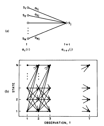
图 4 (a) Illustration of the sequence of operations required for the computation of the forward variable \(\alpha_{t+1}(j)\). (b) Implementation of the computation of \(\alpha_{t}(j)\) in terms of a lattice of observations \(t\), and states \(i\).
If we examine the computation involved in the calculation of \(\alpha_t(j)\), \(1 \leq t \leq T\), \(1 \leq j \leq N\), we see that it requires on the order of \(N^2 T\) calculations, rather than \(2 T N^T\) as required by the direct calculation. (Again, to be precise, we need \(N(N+1)(T-1) + N\) multiplications and \(N(N-1)(T-1)\) additions.) For \(N = 5\), \(T = 100\), we need about \(3000\) computations for the forward method, versus \(10^{72}\) computations for the direct calculation, a savings of about \(69\) orders of magnitude.
The forward probability calculation is, in effect, based upon the lattice (or trellis) structure shown in 图 4 (b). The key is that since there are only \(N\) states (nodes at each time slot in the lattice), all the possible state sequences will re-merge into these \(N\) nodes, no matter how long the observation sequence. At time \(t = 1\) (the first time slot in the lattice), we need to calculate values of \(\alpha_1(i)\), \(1 \leq i \leq N\). At times \(t = 2, 3, \ldots, T\), we only need to calculate values of \(\alpha_t(j)\), \(1 \leq j \leq N\), where each calculation involves only \(N\) previous values of \(\alpha_{t-1}(i)\) because each of the \(N\) grid points is reached from the same \(N\) grid points at the previous time slot.
In a similar manner 7, we can consider a backward variable \(\beta_t(i)\) defined as
i.e., the probability of the partial observation sequence from \(t + 1\) to the end, given state \(S_i\) at time \(t\) and the model \(\lambda\). Again we can solve for \(\beta_t(i)\) inductively, as follows:
Initialization:
(24)¶\[\beta_T(i) = 1, \quad 1 \leq i \leq N.\]Induction:
(25)¶\[\beta_t(i) = \sum_{j = 1}^N a_{ij} b_j(O_{t+1}) \beta_{t+1}(j), \quad t = T-1, T-2, \cdots, 1, \quad 1 \leq i \leq N.\]
The initialization step 1) arbitrarily defines \(\beta_T(i)\) to be \(1\) for all \(i\). Step 2), which is illustrated in 图 5, shows that in order to have been in state \(S_i\) at time \(t\), and to account for the observation sequence from time \(t + 1\) on, you have to consider all possible states \(S_j\) at time \(t + 1\), accounting for the transition from \(S_i\) to \(S_j\) (the \(a_{ij}\) term), and then account for the remaining partial observation sequence from state \(j\) (the \(\beta_{t+1}(j)\) term). We will see later how the backward, as well as the forward calculations are used extensively to help solve fundamental Problems 2 and 3 of HMMs.
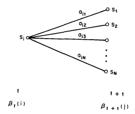
图 5 Illustration of the sequence of operations required for the computation of the backward variable \(\beta_t(i)\).
Again, the computation of \(\beta_t(i)\), \(1 \leq t \leq T\), \(1 \leq i \leq N\), requires on the order of \(N^2 T\) calculations, and can be computed in a lattice structure similar to that of 图 4 (b).
Solution to Problem 2
Unlike Problem 1 for which an exact solution can be given, there are several possible ways of solving Problem 2, namely finding the “optimal” state sequence associated with the given observation sequence. The difficulty lies with the definition of the optimal state sequence; i.e., there are several possible optimality criteria. For example, one possible optimality criterion is to choose the states \(q_t\), which are individually most likely. This optimality criterion maximizes the expected number of correct individual states. To implement this solution to Problem 2, we define the variable
i.e., the probability of being in state \(S_i\) at time \(t\), given the observation sequence \(\mathcal{O}\), and the model \(\lambda\). Equation (26) can be expressed simply in terms of the forward-backward variables, i.e.,
since \(\alpha_t(i)\) accounts for the partial observation sequence \(O_1 O_2 \cdots O_t\) and state \(S_i\) at \(t\), while \(\beta_t(i)\) accounts for the remainder of the observation sequence \(O_{t+1} O_{t+2} \cdots O_T\), given state \(S_i\) at \(t\). The normalization factor \(P(\mathcal{O} \mid \lambda) = \sum_{i=1}^N \alpha_t(i)\), \(\beta_t(i)\) makes \(\gamma_t(i)\) a probability measure so that
Using \(\gamma_t(i)\), we can solve for the individually most likey state \(q_t\) at time \(t\), as
Although (29) maximizes the expected number of correct states (by choosing the most likely state for each \(t\)), there could be some problems with the resulting state sequence. For example, when the HMM has state transitions which have zero probability (\(a_{ij} = 0\) for some \(i\) and \(j\)), the “optimal” state sequence may, in fact, not even be a valid state sequence. This is due to the fact that the solution of (29) simply determines the most likely state at every instant, without regard to the probability of occurrence of sequences of states.
One possible solution to the above problem is to modify the optimality criterion. For example, one could solve for the state sequence that maximizes the expected number of correct pairs of states \((q_t, q_{t + 1})\), or triples of states \((q_t, q_{t + 1}, q_{t+2})\), etc. Although these criteria might be reasonable for some applications, the most widely used criterion is to find the single best state sequence (path), i.e., to maximize \(P(Q \mid \mathcal{O}, \lambda)\) which is equivalent to maximizing \(P(Q, \mathcal{O} \mid \lambda)\). A formal technique for finding this single best state sequence exists, based on dynamic programming methods, and is called the Viterbi algorithm.
Viterbi Algorithm [Ref21], [Ref22]: To find the single best state sequence, \(Q = \{q_1 q_2 \cdots q_T\}\), for the given observation sequence \(O = \{O_1 O_2 \cdots O_T\}\), we need to define the quantity
i.e., \(\delta_t(i)\) is the best score (highest probability) along a single path, at time \(t\), which accounts for the first \(t\) observations and ends in state \(S_i\). By induction we have
To actually retrieve the state sequence, we need to keep track of the argument which maximized (31), for each \(t\) and \(j\). We do this via the array \(\psi_t(j)\). The complete procedure for finding the best state sequence can now be stated as follows:
Initialization:
(32)¶\[\begin{split}\delta_1(i) & = \pi b_i(O_1), \quad 1 \leq i \leq N \\ \psi_1(i) & = 0\end{split}\]Recursion:
(33)¶\[\begin{split}\delta_t(j) & = \mathrm{max}_{1 \leq i \leq N} [\delta_{t-1}(i) a_{ij}] b_j(O_t), \quad 2 \leq t \leq T, \quad 1 \leq j \leq N \\ \psi_t(j) & = \mathrm{argmax}_{1 \leq i \leq N} [\delta_{t-1}(i) a_{ij}], \quad 2 \leq t \leq T, \quad 1 \leq j \leq N.\end{split}\]Termination:
(34)¶\[\begin{split}P^* & = \mathrm{max}_{1 \leq i \leq N} [\delta_T(i)] \\ q_T^* & = \mathrm{argmax}_{1 \leq i \leq N} [\delta_T(i)].\end{split}\]Path (state sequence) backtracking:
It should be noted that the Viterbi algorithm is similar (except for the backtracking step) in implementation to the forward calculation of (19) (20) (21). The major difference is the maximization in (33) (a) over previous states which is used in place of the summing procedure in (20). It also should be clear that a lattice (or trellis) structure efficiently implements the computation of the Viterbi procedure.
Solution to Problem 3 [Ref1] - [Ref5]
The third, and by far the most difficult, problem of HMMs is to determine a method to adjust the model parameters \((A, B, \pi)\) to maximize the probability of the observation sequence given the model. There is no known way to analytically solve for the model which maximizes the probability of the observation sequence. In fact, given any finite observation sequence as training data, there is no optimal way of estimating the model parameters. We can, however, choose \(\lambda = (A, B, \pi)\) such that \(P(\mathcal{O} \mid \lambda)\) is locally maximized using an iterative procedure such as the Baum-Welch method (or equivalently the EM (expectation-modification) method [Ref23]), or using gradient techniques [Ref14]. In this section we discuss one iterative procedure, based primarily on the classic work of Baum and his colleagues, for choosing model parameters.
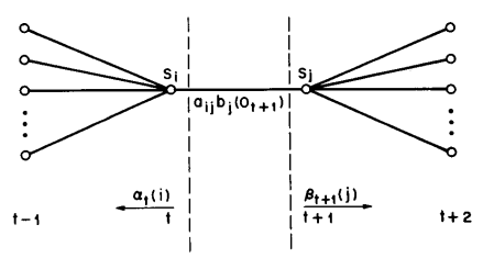
图 6 Illustration of the sequence of operations required for the computation of the joint event that the system is in state \(S_i\), at time \(t\) and state \(S_j\), at time \(t + 1\).
In order to describe the procedure for reestimation (iterative update and improvement) of HMM parameters, we first define \(\xi_t(i, j)\), the probability of being in state \(S_i\) at time \(t\), and state \(S_j\), at time \(t+1\), given the model and the observation sequence, i.e.
The sequence of events leading to the conditions required by (36) is illustrated in 图 6. It should be clear, from the definitions of the forward and backward variables, that we can write \(\xi_t(i, j)\) in the form
where the numerator term is just \(P(q_t = S_i, q_{t+1} = S_j, \mathcal{O} \mid \lambda)\) and division by \(P(\mathcal{O} \mid \lambda)\) gives the desired probability measure.
We have previously defined \(\gamma_t(i)\) as the probability of being in state \(S_i\) at time \(t\), given the observation sequence and the model; hence we can relate \(\gamma_t(i)\) to \(\xi_t(i, j)\) by summing over \(j\), giving
If we sum \(\gamma_t(i)\) over the time index \(t\), we get a quantity which can be interpreted as the expected (over time) number of times that state \(S_i\) is visited, or equivalently, the expected number of transitions made from state \(S_i\) (if we exclude the time slot \(t = T\) from the summation). Similarly, summation of \(\xi_t(i, j)\) over \(t\) (from \(t = 1\) to \(t = T - 1\)) can be interpreted as the expected number of transitions from state \(S_i\) to state \(S_j\). That is
Using the above formulas (and the concept of counting event occurrences) we can give a method for reestimation of the parameters of an HMM. A set of reasonable reestimation formulas for \(\pi\), \(A\), and \(B\) are
If we define the current model as \(\lambda = (A, B, \pi)\), and use that to compute the right-hand sides of (40), and we define the reestimated model as \(\bar{\lambda} = (\bar{A}, \bar{B}, \bar{\pi})\), as determined from the left-hand sides of (40), then it has been proven by Baum and his colleagues [Ref6], [Ref3] that either 1) the initial model \(\lambda\) defines a critical point of the likelihood function, in which case \(\bar{\lambda} = \lambda\); or 2) model \(\bar{\lambda}\) is more likely than model \(\lambda\) in the sense that \(P(\mathcal{O} \mid \bar{\lambda}) > P(\mathcal{O} \mid \lambda)\), i.e., we have found a new model \(\bar{\lambda}\) from which the observation sequence is more likely to have been produced.
Based on the above procedure, if we iteratively use \(\bar{\lambda}\) in place of \(\lambda\) and repeat the reestimation calculation, we then can improve the probability of \(\mathcal{O}\) being observed from the model until some limiting point is reached. The final result of this reestimation procedure is called a maximum likelihood estimate of the HMM. It should be pointed out that the forward-backward algorithm leads to local maxima only, and that in most problems of interest, the optimization surface is very complex and has many local maxima.
The reestimation formulas of (40) can be derived directly by maximizing (using standard constrained optimization techniques) Baum’s auxiliary function
over \(\bar{\lambda}\). It has been proven by Baum and his colleagues [Ref6], [Ref3] that maximization of \(Q(\lambda, \bar{\lambda})\) leads to increased likelihood, i.e.
Eventually the likelihood function converges to a critical point.
Notes on the Reestimation Procedure: The reestimation formulas can readily be interpreted as an implementation of the EM algorithm of statistics [Ref23] in which the E (expectation) step is the calculation of the auxiliary function \(Q(\lambda, \bar{\lambda})\), and the M (modification) step is the maximization over \(\bar{\lambda}\). Thus the Baum-Welch reestimation equations are essentially identical to the EM steps for this particular problem.
An important aspect of the reestimation procedure is that the stochastic constraints of the HMM parameters, namely
are automatically satisfied at each iteration. By looking at the parameter estimation problem as a constrained optimization of \(P(\mathcal{O} \mid \lambda)\) (subject to the constraints of (43)), the techniques of Lagrange multipliers can be used to find the values of \(\pi, a_{ij}\) and \(b_j(k)\) which maximize \(P\) (we use the notation \(P = P(\mathcal{O} \mid \lambda)\) as short-hand in this section). Based on setting up a standard Lagrange optimization using Lagrange multipliers, it can readily be shown that \(P\) is maximized when the following conditions are met:
By appropriate manipulation of (44), the right-hand sides of each equation can be readily converted to be identical to the right-hand sides of each part of (40), thereby showing that the reestimation formulas are indeed exactly correct at critical points of \(P\). In fact the form of (44) is essentially that of a reestimation formula in which the left-hand side is the reestimate and the right-hand side is computed using the current values of the variables.
Finally, we note that since the entire problem can be set up as an optimization problem, standard gradient techniques can be used to solve for “optimal” values of the model parameters [Ref14]. Such procedures have been tried and have been shown to yield solutions comparable to those of the standard reestimation procedures.
TYPES OF HMMs
Until now, we have only considered the special case of ergodic or fully connected HMMs in which every state of the model could be reached (in a single step) from every other state of the model. (Strictly speaking, an ergodic model has the property that every state can be reached from every other state in a finite number of steps.) As shown in 图 7 (a), for an \(N = 4\) state model, this type of model has the property that every \(a_{ij}\) coefficient is positive. Hence for the example of 图 7 (a) we have
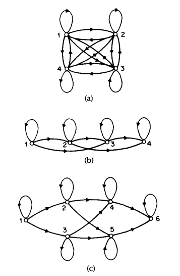
图 7 Illustration of 3 distinct types of HMMs. (a) A 4-state ergodic model. (b) A 4-state left-right model. (c) A 6-state parallel path left-right model.
For some applications, in particular those to be discussed later in this paper, other types of HMMs have been found to account for observed properties of the signal being modeled better than the standard ergodic model. One such model is shown in 图 7 (b). This model is called a left-right model or a Bakis model [Ref11], [Ref10] because the underlying state sequence associated with the model has the property that as time increases the state index increases (or stays the same), i.e., the states proceed from left to right. Clearly the left-right type of HMM has the desirable property that it can readily model signals whose properties change overtime- e.g., speech. The fundamental property of all left-right HMMs is that the state transition coefficients have the property
i.e., no transitions are allowed to states whose indices are lower than the current state. Furthermore, the initial state probabilities have the property
since the state sequence must begin in state \(1\) (and end in state \(N\)) . Often, with left-right models, additional constraints are placed on the state transition coefficients to make sure that large changes in state indices do not occur; hence a constraint of the form
is often used. In particular, for the example of 图 7 (b), the value of \(\Delta\) is \(2\), i.e., no jumps of more than \(2\) states are allowed. The form of the state transition matrix for the example of 图 7 (b) is thus
It should be clear that, for the last state in a left-right model, that the state transition coefficients are specified as
Although we have dichotomized HMMs into ergodic and left-right models, there are many possible variations and combinations possible. By way of example, 图 7 (c) shows a cross-coupled connection of two parallel left-right HMMs. Strictly speaking, this model is a left-right model (it obeys all the \(a_{ij}\) constraints); however, it can be seen that it has certain flexibility not present in a strict left-right model (i.e., one without parallel paths).
It should be clear that the imposition of the constraints of the left-right model, or those of the constrained jump model, essentially have no effect on the reestimation procedure. This is the case because any HMM parameter set to zero initially, will remain at zero throughout the reestimation procedure (see (44)).
Continuous Observation Densities in HMMs [Ref24], [Ref25], [Ref26]
All of our discussion, to this point, has considered only the case when the observations were characterized as discrete symbols chosen from a finite alphabet, and therefore we could use a discrete probability density within each state of this model. The problem with this approach, at least for some applications, is that the observations are continuous signals (or vectors). Although it is possible to quantize such continuous signals via codebooks, etc., there might be serious degradation associated with such quantization. Hence it would be advantageous to be able to use HMMs with continuous observation densities.
In order to use a continuous observation density, some restrictions have to be placed on the form of the model probability density function (pdf) to insure that the parameters of the pdf can be reestimated in a consistent way. The most general representation of the pdf, for which a reestimation procedure has been formulated [Ref24], [Ref25], [Ref26], is a finite mixture of the form
where \(\mathbf{O}\) is the vector being modeled, \(c_{jm}\) is the mixture coefficient for the \(m\) -th mixture in state \(j\) and \(\mathcal{N}\) is any log-concave or elliptically symmetric density [Ref24] (e.g., Gaussian), with mean vector \(\mu_{jm}\) and covariance matrix \(\mathbf{U}_{jm}\) for the \(m\) -th in state \(j\). Usually a Gaussian density is used for \(\mathcal{N}\). The mixture gains \(c_{jm}\) satisfy the stochastic constraint
so that the pdf is properly normalized, i.e.,
The pdf of (49) can be used to approximate, arbitrarily closely, any finite, continuous density function. Hence it can be applied to a wide range of problems.
It can be shown [Ref24], [Ref25], [Ref26] that the reestimation formulas for the coefficients of the mixture density, i.e., \(c_{jm}, \mu_{jk}\), and \(\mathbf{U}_{jk}\), are of the form
where prime denotes vector transpose and where \(\gamma_t(j, k)\) is the probability of being in state \(j\) at time \(t\) with the \(k\) -th mixture component accounting for \(\mathbf{O}_t\), i.e.,
(The term \(\gamma_t(j, k)\) generalizes to \(\gamma_t(j)\) of (26) in the case of a simple mixture, or a discrete density.) The reestimation formula for \(a_{ij}\) is identical to the one used for discrete observation densities (i.e., (40)). The interpretation of (52), (53), (54) is fairly straightforward. The reestimation formula for \(c_{jk}\) is the ratio between the expected number of times the system is in state \(j\) using the \(k\) -th mixture component, and the expected number of times the system is in state \(j\). Similarly, the reestimation formula for the mean vector \(\mu_{jk}\) weights each numerator term of (52) by the observation, thereby giving the expected value of the portion of the observation vector accounted for by the \(k\) -th mixture component. A similar interpretation can be given for the reestimation term for the covariance matrix \(\mathbf{U}_{jk}\).
Autoregressive HMMs [Ref27], [Ref28]
Although the general formulation of continuous density HMMs is applicable to a wide range of problems, there is one other very interesting class of HMMs that is particularly applicable to speech processing. This is the class of autoregressive HMMs [Ref27], [Ref28]. For this class, the observation vectors are drawn from an autoregression process.
To be more specific, consider the observation vector \(\mathbf{O}\) with components \((x_0, x_1, x_2, \ldots, x_{K-1})\). Since the basis probability density function for the observation vector is Gaussian autoregressive (or order \(p\)), then the components of \(\mathbf{O}\) are related by
where \(e_k, k = 0, 1, 2, \ldots, K - 1\) are Gaussian, independent, identically distributed random variables with zero mean and variance \(\sigma^2\), and \(a_i, i = 1, 2, \ldots, p\), are the autoregression or predictor coefficients. It can be shown that for large \(K\), the density function for \(\mathbf{O}\) is approximately
where
In the above equations it can be recognized that \(r(i)\) is the autocorrelation of the observation samples, and \(r_a(i)\) is the autocorrelation of the autoregressive coefficients.
The total (frame) prediction residual \(\alpha\) can be written as
where \(\sigma^2\) is the variance per sample of the error signal. Consider the normalized observation vector
where each sample \(x_i\), is divided by \(\sqrt{K \sigma^2}\), i.e., each sample is normalized by the sample variance. Then \(f(\hat{\mathbf{O}})\) can be written as
In practice, the factor \(K\) (in front of the exponential of (60)) is replaced by an effective frame length \(K\) which represents the effective length of each data vector. Thus if consecutive data vectors are overlapped by 3 to 1, then we would use \(\hat{K} = K/3\) in (60), so that the contribution of each sample of signal to the overall density is counted exactly once.
The way in which we use Gaussian autoregressive density in HMMs is straightforward. We assume a mixture density of the form
where each \(b_{jm}(\mathbf{O})\) is the density defined by (60) with autoregression vector \(a_{jm}\) (or equivalently by autocorrelation vector \(r_{a_{jm}}\)), i.e.,
A reestimation formula for the sequence autocorrelation, \(r(i)\) of (57), for the \(j\) -th state, \(k\) th mixture, component has been derived, and is of the form
where \(\gamma_t(j, k)\) is defined as the probability of being in state \(j\) at time \(t\) and using mixture component \(k\), i.e.,
It can be seen that \(\bar{\mathbf{r}}_{jk}\) is a weighted sum (by probability of occurrence) of the normalized autocorrelations of the frames in the observation sequence. From \(\bar{\mathbf{r}}_{jk}\), one can solve a set of normal equations to obtain the corresponding autoregressive coefficient vector \(\bar{\mathbf{a}}_{jk}\), for the \(k\) -th mixture of state \(j\). The new autocorrection vectors of the autoregression coefficients can then be calculated using (57), thereby closing the reestimation loop.
Variants on HMM Structures - Null Transitions and Tied States
Throughout this paper we have considered HMMs in which the observations were associated with states of the model. It is also possible to consider models in which the observations are associated with the arcs of the model. This type of HMM has been used extensively in the IBM continuous speech recognizer [Ref13]. It has been found useful, for this type of model, to allow transitions which produce no output-i.e., jumps from one state to another which produce no observation [Ref13]. Such transitions are called null transitions and are designated by a dashed line with the symbol \(\phi\) used to denote the null output.
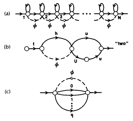
图 8 Examples of networks incorporating null transitions. (a) Left-right model. (b) Finite state network. (c) Grammar network.
图 8 illustrates 3 examples (from speech processing tasks) where null arcs have been successfully utilized. The example of part (a) corresponds to an HMM (a left-right model) with a large number of states in which it is possible to omit transitions between any pair of states. Hence it is possible to generate observation sequences with as few as \(1\) observation and still account for a path which begins in state \(1\) and ends in state \(N\).
The example of 图 8 (b) is a finite state network (FSN) representation of aword in terms of linguistic unit models (i.e., the sound on each arc is itself an HMM). For this model the null transition gives a compact and efficient way of describing alternate word pronunciations (i.e., symbol delections).
Finally the FSN of 图 8 (c) shows how the ability to insert a null transition into a grammar network allows a relatively simple network to generate arbitrarily long word (digit) sequences. In the example shown in 图 8 (c), the null transition allows the network to generate arbitrary sequences of digits of arbitrary length by returning to the initial state after each individual digit is produced.
Another interesting variation in the HMM structure is the concept of parameter tieing [Ref13]. Basically the idea is to set up an equivalence relation between HMM parameters in different states. In this manner the number of independent parameters in the model is reduced and the parameter estimation becomes somewhat simpler. Parameter tieing is used in cases where the observation density (for example) is known to be the same in 2 or more states. Such cases occur often in characterizing speech sounds. The technique is especially appropriate in the case where there is insufficient training data to estimate, reliably, a large number of model parameters. For such cases it is appropriate to tie model parameters so as to reduce the number of parameters (i.e., size of the model) thereby making the parameter estimation problem somewhat simpler. We will discuss this method later in this paper.
Inclusion of Explicit State Duration Density in HMMs 8, [Ref29], [Ref30]
Perhaps the major weakness of conventional HMMs is the modeling of state duration. Earlier we showed (5) that the inherent duration probability density \(p_i(d)\) associated with state \(S_i\), with self transition coefficient \(a_{ii}\), was of the form
For most physical signals, this exponential state duration density is inappropriate. Instead we would prefer to explicitly model duration density in some analytic form. 图 9 illustrates, for a pair of model states \(S_i\) and \(S_j\), the differences between HMMs without and with explicit duration density. In part (a) the states have exponential duration densities based on self-transition coefficients \(a_{ii}\) and \(a_{jj}\), respectively. In part (b), the self-transition coefficients are set to zero, and an explicit duration density is specified 9. For this case, a transition is made only after the appropriate number of observations have occurred in the state (as specified by the duration density).
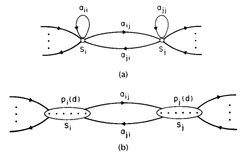
图 9 Illustration of general interstate connections of (a) a normal HMM with exponential state duration density, and (b) a variable duration HMM with specified state densities and no self transitions from a state back to itself.
Based on the simple model of 图 9 (b), the sequence of events of the variable duration HMM is as follows:
An initial state, \(q_1 = S_i\), is chosen according to the initial state distribution \(\pi_i\).
A duration \(d_1\) is chosen according to the state duration density \(p_{q_1}(d_1)\). (For expedience and ease of implementation the duration density \(p_q(d)\) is truncated at a maximum duration value \(D\).)
Observations \(O_1 O_2 \cdots O_{d_1}\) are chosen according to the joint observation density, \(b_{q_1}(O_1 O_2 \cdots O_{d_1})\). Generally we assume independent of observations so that \(b_{q_1}(O_1 O_2 \cdots O_{d_1}) = \prod_{t = 1}^{d_1} b_{q_1}(O_t)\).
The next state, \(q_2 = S_j\), is chosen according to the state transition probabilities, \(a_{q_1 q_2}\), with the constraint that \(a_{q_1 q_2} = 0\), i.e., no transition back to the same state can occur. (Clearly this is a requirement since we assume that, in state \(q_1\), exactly \(d_1\) observations occur.)
A little thought should convince the reader that the variable duration HMM can be made equivalent to the standard HMM by setting \(p_i(d)\) to be the exponential density of (65).
Using the above formulation, several changes must be made to the formulas of Section III to allow calculation of \(P(\mathcal{O} \mid \lambda)\) and for reestimation of all model parameters. In particular we assume that the first state begins at \(t = 1\) and the last state ends at \(t = T\), i.e., entire duration intervals are included with the observation sequence. We then define the forward variable \(\alpha_t(i)\) as
We assume that a total of \(r\) states have been visited during the first \(t\) observations and we denote the states as \(q_1, q_2, \ldots, q_r\), with durations associated with each state of \(d_1, d_2, \ldots, d_r\) Thus the constraints of (66) are
Equation (66) can then be written as
where the sum is over all states \(q\) and all possible state durations \(d\). By induction we can write \(\alpha_t(j)\) as
where \(D\) is the maximum duration within any state. To initialize the computation of \(\alpha_t(j)\) we use
etc., until \(\alpha_D(i)\) is computed; then (69) can be used for all \(t > D\). It should be clear that the desired probability of \(\mathcal{O}\) given the model \(\lambda\) can be written in terms of the \(\alpha\)’s as
as was previously used for ordinary HMMs.
In ordertogive reestimation formulas for all the variables of the variable duration HMM, we must define three more forward-backward variables, namely
The relationships between \(\alpha, \alpha^*, \beta,\) and \(\beta^*\) are as follows:
Based on the above relationships and definitions, the reestimation formulas for the variable duration HMM are
The interpretation of the reestimation formulas is the following. The formula for \(\bar{\pi}_i\) is the probability that state \(i\) was the first state, given \(\mathcal{O}\). The formula for \(\bar{a}_{ij}\) is almost the same as for the usual HMM except it uses the condition that the alpha terms in which a state ends at \(t\), join with the beta terms in which a new state begins at \(t + 1\). The formula for \(\bar{b}_i(k)\) (assuming a discrete density) is the expected number of times that observation \(O_t = v_k\) occurred in state \(i\), normalized by the expected number of times that any observation occurred in state \(i\). Finally, the reestimation formula for \(\bar{p}_i(d)\) is the ratio of the expected number of times state \(i\) occurred with duration \(d\), to the expected number of times state \(i\) occurred with any duration.
The importance of incorporating state duration densities is reflected in the observation that, for some problems, the quality of the modeling is significantly improved when explicit state duration densities are used. However, there are drawbacks to the use of the variable duration model discussed in this section. One is the greatly increased computational load associated with using variable durations. It can be seen from the definition and initialization conditions on the forward variable \(\alpha_i(i)\), from (69), (70), that about \(D\) times the storage and \(D^2/2\) times the computation is required. For \(D\) on the order of 25 (as is reasonable for many speech processing problems), computation is increased by a factor of 300. Another problem with the variable duration models is the large number of parameters (\(D\)), associated with each state, that must be estimated, in addition to the usual HMM parameters. Furthermore, for a fixed number of observations \(T\), in the training set, there are, on average, fewer state transitions and much less data to estimate \(p_i(d)\) than would be used in a standard HMM. Thus the reestimation problem is more difficult for variable duration HMMs than for the standard HMM.
One proposal to alleviate some of these problems is to use a parametric state duration density instead of the non-parametric \(p_i(d)\) used above [Ref29], [Ref30]. In particular, proposals include the Gaussian family with
with parameters \(\mu_i\) and \(\sigma_i^2\), or the Gamma family with
with parameters \(\nu_i\) and \(\eta_i\) and with mean \(\nu_i \eta_i^{-1}\) and variance \(\nu_i \eta_i^{-2}\). Reestimation formulas for \(\eta_i\) and \(\nu_i\) have been derived and used with good results [Ref19]. Another possibility, which has been used with good success, is to assume a uniform duration distribution (over an appropriate range of durations) and use a path-constrained Viterbi decoding procedure [Ref31].
Optimization Criterion - ML, MMI, and MDI [Ref32], [Ref33]
The basic philosophy of HMMs is that a signal (or observation sequence) can be well modeled if the parameters of an HMM are carefully and correctly chosen. The problem with this philosophy is that it is sometimes inaccurate - either because the signal does not obey the constraints of the HMM, or because it is too difficult to get reliable estimates of all HMM parameters. To alleviate this type of problem, there has been proposed at least two alternatives to the standard maximum likelihood (ML) optimization procedure for estimating HMM parameters.
The first alternative [Ref32] is based on the idea that several HMMs are to be designed and we wish to design them all at the same time in such a way so as to maximize the discrimination power of each model (i.e., each model’s ability to distinguish between observation sequences generated by the correct model and those generated by alternative models). We denote the different HMMs as \(\lambda_{\nu}, \nu = 1, 2, \ldots, V\). The standard ML design criterion is to use a separate training sequence of observations \(O^{\nu}\) to derive model parameters for each model \(\lambda_{\nu}\). Thus the standard ML optimization yields
The proposed alternative design criterion [Ref31] is the maximum mutual information (MMI) criterion in which the average mutual information \(I\) between the observation sequence \(O^{\nu}\) and the complete set of models \(\lambda = (\lambda_1, \lambda_2, \ldots, \lambda_V)\) is maximized. One possible way of implementing this 10 is
i.e., choose \(\lambda\) so as to separate the correct model \(\lambda_{\nu}\), from all other models on the training sequence \(O^{\nu}\). By summing (86) over all training sequences, one would hope to attain the most separated set of models possible. Thus a possible implementation would be
There are various theoretical reasons why analytical (or reestimation type) solutions to (87) cannot be realized. Thus the only known way of actually solving (87) is via general optimization procedures like the steepest descent methods [Ref32].
The second alternative philosophy is to assume that the signal to be modeled was not necessarily generated by a Markov source, but does obey certain constraints (e.g., positive definite correlation function) [Ref33]. The goal of the design procedure is therefore to choose HMM parameters which minimize the discrimination information (DI) or the cross entropy between the set of valid (i.e., which satisfy the measurements) signal probability densities (call this set \(Q\)), and the set of HMM probability densities (call this set \(P_{\lambda}\)), where the DI between \(Q\) and \(P_{\lambda}\) can generally be written in the form
where \(q\) and \(p\) are the probability density functions corresponding to \(Q\) and \(P_{\lambda}\). Techniques for minimizing (88) (thereby giving an MDI solution) for the optimum values of \(\lambda = (A, B, \pi)\) are highly nontrivial; however, they use a generalized Baum algorithm as the core of each iteration, and thus are efficiently tailored to hidden Markov modeling [Ref33].
It has been shown that the ML, MMI, and MDI approaches can all be uniformly formulated as MDI approaches. 11 The three approaches differ in either the probability density attributed to the source being modeled, or in the model effectively being used. None of the approaches, however, assumes that the source has the probability distribution of the model.
Comparison of HMMs [Ref34]
An interesting question associated with HMMs is the following: Given two HMMs, \(\lambda_1\) and \(\lambda_2\), what is a reasonable measure of the similarity of the two models? A key point here is the similarity criterion. By way of example, consider the case of two models
with
and
For \(\lambda_1\) to be equivalent to \(\lambda_2\), in the sense of having the same statistical properties for the observation symbols, i.e., \(E[O_t = v_k \mid \lambda_1] = E[O_t = v_k \mid \lambda_2]\) for all \(v_k\), we require
or, by solving for \(s\), we get
By choosing (arbitrarily) \(p = 0.6, q = 0.7, r = 0.2\), we get \(s= 13/30 \approx 0.433\). Thus, even when the two models, \(\lambda_1\), and \(\lambda_2\), look ostensibly very different (i.e., \(A_1\) is very different from \(A_2\), and \(B_1\) is very different from \(B_2\)), statistical equivalence of the models can occur.
We can generalize the concept of model distance (dissimilarity) by defining a distance measure \(D(\lambda_1, \lambda_2)\), between two Markov models, \(\lambda_1\), and \(\lambda_2\), as
where \(O^{(2)} = O_1 O_2 O_3 \cdots O_T\) is a sequence of observations generated by model \(\lambda_2\) [Ref34]. Basically (89) is a measure of how well model \(\lambda_1\) matches observations generated by model \(\lambda_2\), relative to how well model \(\lambda_2\) matches observations generated by itself. Several interpretations of (89) exist in terms of cross entropy, or divergence, or discrimination information [Ref34].
One of the problems with the distance measure of (89) is that it is nonsymmetric. Hence a natural expression of this measure is the symmetrized version, namely
IMPLEMENTATION ISSUES FOR HMMs
The discussion in the previous two sections has primarily dealt with the theory of HMMs and several variations on the form of the model. In this section we deal with several practical implementation issues including scaling, multiple observation sequences, initial parameter estimates, missing data, and choice of model size and type. For some of these implementation issues we can prescribe exact analytical solutions; for other issues we can only provide some seat-of-the-pants experience gained from working with HMMs over the last several years.
Scaling [Ref14]
In order to understand why scaling is required for implementing the reestimation procedure of HMMs, consider the definition of \(\alpha_t(i)\) of (18). It can be seen that \(\alpha_t(i)\) consists of the sum of a large number of terms, each of the form
with \(q_t = S_i\). Since each \(a\) and \(b\) term is less than 1 (generally significantly less than 1), it can be seen that as \(t\) starts to get big (e.g., 10 or more), each term of \(\alpha_t(i)\) starts to head exponentially to zero. For sufficiently large \(t\) (e.g., 100 or more) the dynamic range of the \(\alpha_t(i)\) computation will exceed the precision range of essentially any machine (even in double precision). Hence the only reasonable way of performing the computation is by incorporating a scaling procedure.
The basic scaling procedure which is used is to multiply \(\alpha_t(i)\) by a scaling coefficient that is independent of \(i\) (i.e., it depends only on \(t\)), with the goal of keeping the scaled \(\alpha_t(i)\) within the dynamic range of the computer for \(1 \leq t \leq T\). A similar scaling is done to the \(\beta_t(i)\) coefficients (since these also tend to zero exponentially fast) and then, at the end of the computation, the scaling coefficients are canceled out exactly.
To understand this scaling procedure better, consider the reestimation formula for the state transition coefficients \(a_{ij}\). If we write the reestimation formula (41) directly in terms of the forward and backward variables we get
Consider the computation of \(\alpha_t(i)\). For each \(t\), we first compute \(\alpha_t(i)\) according to the induction formula (20), and then we multiply it by a scaling coefficient \(c_t\), where
Thus, for a fixed \(t\), we first compute
Then the scaled coefficient set \(\hat{\alpha}_t(i)\) is computed as
By induction we can write \(\hat{\alpha}_{t-1}(j)\) as
Thus we can write \(\hat{\alpha}_{t}(i)\) as
i.e., each \(\alpha_t(i)\) is effectively scaled by the sum over all states of \(\alpha_t(i)\).
Next we compute the \(\beta_t(i)\) terms from the backward recursion. The only difference here is that we use the same scale factors for each time \(t\) for the betas as was used for the alphas. Hence the scaled \(\beta\)’s are of the form
Since each scale factor effectively restores the magnitude of the \(\alpha\) terms to 1, and since the magnitudes of the \(\alpha\) and \(\beta\) terms are comparable, using the same scaling factors on the \(\beta\)’s as was used on the \(\alpha\)’s is an effective way of keeping the computation within reasonable bounds. Furthermore, in terms of the scaled variables we see that the reestimation equation (91) becomes
but each \(\hat{\alpha}_t(i)\) can be written as
and each \(\hat{\beta}_{t+1}(j)\) can be written as
Thus (98) can be written as
Finally the term \(C_t D_{t+1}\) can be seen to be of the form
independent of \(t\). Hence the terms \(C_t D_{t+1}\) cancel out of both the numerator and denominator of (101) and the exact reestimation equation is therefore realized.
It should be obvious that the above scaling procedure applies equally well to reestimation of the \(\pi\) or \(B\) coefficients. It should also be obvious that the scaling procedure of (93) and (94) need not be applied at every time instant \(t\), but can be performed whenever desired, or necessary (e.g., to prevent underflow). If scaling is not performed at some instant \(t\), the scaling coefficients \(c_t\), are set to \(1\) at that time and all the conditions discussed above are then met.
The only real change to the HMM procedure because of scaling is the procedure for computing \(P(O \mid \lambda)\). We cannot merely sum up the \(\hat{\alpha_T(i)}\) terms since these are scaled already. However, we can use the property that
Thus we have
or
or
Thus the log of \(P\) can be computed, but not \(P\) since it would be out of the dynamic range of the machine anyway.
Finally we note that when using the Viterbi algorithm to give the maximum likelihood state sequence, no scaling is required if we use logarithms in the following way. (Refer back to (32), (33), (34).) We define
and initially set
with the recursion step
and termination step
Again we arrive at \(\log P^*\) rather than \(P^*\), but with significantly less computation and with no numerical problems. (The reader should note that the terms \(\log a_{ij}\), of (109) can be precomputed and therefore do not cost anything in the computation. Furthermore, the terms \(\log b_j(O_t)\) can be precomputed when a finite observation symbol analysis (e.g., a codebook of observation sequences) is used.
Multiple Observation Sequences [Ref14]
In Section IV we discussed a form of HMM called the left-right or Bakis model in which the state proceeds from state 1 at \(t = 1\) to state \(N\) at \(t = T\) in a sequential manner (recall the model of 图 7 (b)). We have already discussed how a left-right model imposes constraints on the state transition matrix, and the initial state probabilities (45) - (48). However, the major problem with left-right models is that one cannot use a single observation sequence to train the model (i.e., for reestimation of model parameters). This is because the transient nature of the states within the model only allow a small number of observations for any state (until a tran- sition is made to a successor state). Hence, in order to have sufficient data to make reliable estimates of all model parameters, one has to use multiple observation sequences.
The modification of the reestimation procedure is straightforward and goes as follows. We denote the set of \(K\) observation sequences as
where \(\mathbf{O}^{(k)} = [O_1^{(k)} O_2^{(2)} \cdots O_{T_k}^{(k)}]\) is the \(k\)-th observation sequence. We assume each observation sequence is independent of every other observation sequence, and our goal is to adjust the parameters of the model \(\lambda\) to maximize
Since the reestimation formulas are based on frequencies of occurrence of various events, the reestimation formulas for multiple observation sequences are modified by adding together the individual frequencies of occurrence for each sequence. Thus the modified reestimation formulas for \(\bar{a}_{ij}\) and \(\bar{b}_j(\ell)\) are
and
and \(\pi\) is not reestimated since \(\pi_1 = 1, \pi_i = 0, i \neq 1\).
The proper scaling of (113) - (114) is now straightforward since each observation sequence has its own scaling factor. The key idea is to remove the scaling factor from each term before summing. This can be accomplished by writing the reestimation equations in terms of the scaled variables, i.e.,
In this manner, for each sequence \(O^{(k)}\), the same scale factors will appear in each term of the sum over \(t\) as appears in the \(P_k\) term, and hence will cancel exactly. Thus using the scaled values of the alphas and betas results in an unscaled \(\bar{a}_{ij}\). A similar result is obtained for the \(\bar{b}_j(\ell)\) term.
Initial Estimates of HMM Parameters
In theory, the reestimation equations should give values of the HMM parameters which correspond to a local maximum of the likelihood function. A key question is therefore how do we choose initial estimates of the HMM parameters so that the local maximum is the global maximum of the likelihood function.
Basically there is no simple or straightforward answer to the above question. Instead, experience has shown that either random (subject to the stochastic and the nonzero value constraints) or uniform initial estimates of the \(\pi\) and \(A\) parameters is adequate for giving useful reestimates of these parameters in almost all cases. However, for the \(B\) parameters, experience has shown that good initial estimates are helpful in the discrete symbol case, and are essential (when dealing with multiple mixtures) in the continuous distribution case [Ref35]. Such initial estimates can be obtained in a number of ways, including manual segmentation of the observation sequence(s) into states with averaging of observations within states, maximum likelihood segmentation of observations with averaging, and segmental \(k\)-means segmentation with clustering, etc. We discuss such segmentation techniques later in this paper.
Effects of Insufficient Training Data [Ref36]
Another problem associated with training HMM parameters via reestimation methods is that the observation sequence used for training is, of necessity, finite. Thus there is often an insufficient number of occurrences of different model events (e.g., symbol occurrences within states) to give good estimates of the model parameters. One solution to this problem is to increase the size of the training observation set. Often this is impractical. A second possible solution is to reduce the size of the model (e.g., number of states, number of symbols per state, etc). Although this is always possible, often there are physical reasons why a given model is used and therefore the model size cannot be changed. A third possible solution is to interpolate one set of parameter estimates with another set of parameter estimates from a model for which an adequate amount of training data exists [Ref36]. The idea is to simultaneously design both the desired model as well as a smaller model for which the amount of training data is adequate to give good parameter estimates, and then to interpolate the parameter estimates from the two models. The way in which the smaller model is chosen is by tieing one or more sets of parameters of the initial model to create the smaller model. Thus if we have estimates for the parameters for the model \(\lambda = (A, B, \pi)\), as well as for the reduced size model \(\lambda^{\prime} = (A^{\prime}, B^{\prime}, K^{\prime})\), then the interpolated model, \(\tilde{\lambda} = (\tilde{A}, \tilde{B}, \tilde{\pi})\), is obtained as
where \(\epsilon\) represents the weighting of the parameters of the full model, and \((1 - \epsilon)\) represents the weighting of the parameters of the reduced model. A key issue is the determination of the optimal value of \(\epsilon\), which is clearly a function of the amount of training data. (As the amount of training data gets large, we expect \(\epsilon\) to tend to \(1.0\); similarly for small amounts of training data we expect \(\epsilon\) to tend to \(0.0\).) The solution to the determination of an optimal value for \(\epsilon\) was provided by Jelinek and Mercer [Ref36] who showed how the optimal value for \(\epsilon\) could be estimated using the forward-backward algorithm by interpreting (116) as an expanded HMM of the type shown in 图 10. For this expanded model the parameter \(\epsilon\) is the probability of a state transition from the (neutral) state \(\tilde{s}\) to the model \(\lambda\); similarly \((1 - \epsilon)\) is the probability of a state transition from \(\tilde{s}\) to the model \(\lambda^{\prime}\). Between each of the models, \(\lambda\) and \(\lambda^{\prime}\), and \(\tilde{s}\), there is a null transition. Using the model of 图 9, the value of \(\epsilon\) can be estimated from the training data in the standard manner. A key point is to segment the training data \(T\) into two disjoint sets, i.e., \(T = T_1 \cup T_2\). Training set \(T_1\) is first used to train models \(\lambda\) and \(\lambda^{\prime}\) (i.e., to give estimates of \((A, B, \pi)\) and \((A^{\prime}, B^{\prime}, \pi^{\prime})\). Training set \(T_2\) is then used to give an estimate of \(\epsilon\), assuming the models \(\lambda\) and \(\lambda^{\prime}\) are fixed. A modified version of this training procedure, called the method of deleted interpolation [Ref36], iterates the above procedure through multiple partitions of the training set. For example one might consider a partition of the training set such that \(T_1\) is 90 percent of \(T\) and \(T_2\) is the remaining 10 percent of \(T\). There are a large number of ways in which such a partitioning can be accomplished but one particularly simple one is to cycle \(T_2\) through the data, i.e., the first partition uses the last 10 percent of the data as \(T_2\), the second partition uses the next-to-last 10 percent of the data as \(T_2\), etc.
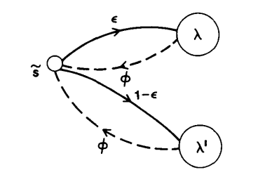
图 10 Example of how the process of deleted interpolation can be represented using a state diagram.
The technique of deleted interpolation has been successfully applied to a number of problems in speech recognition including the estimation of trigram word probabilities for language models [Ref13], and the estimation of HMM output probabilities for trigram phone models [Ref37], [Ref38].
Another way of handling the effects of insufficient training data is to add extra constraints to the model parameters to insure that no model parameter estimate falls below a specified level. Thus, for example, we might specify the constraint, for a discrete symbol model, that
or, for a continuous distribution model, that
The constraints can be applied as a postprocessor to the reestimation equations such that if a constraint is violated, the relevant parameter is manually corrected, and all remaining parameters are rescaled so that the densities obey the required stochastic constraints. Such post-processor techniques have been applied to several problems in speech processing with good success [Ref39]. It can be seen from (116) that this procedure is essentially equivalent to a simple form of deleted interpolation in which the model \(\lambda^{\prime}\) is a uniform distribution model, and the interpolation value \(\epsilon\) is chosen as the fixed constant \((1 - \delta)\).
Choice of Model
The remaining issue in implementing HMMs is the choice of type of model (ergodic or left-right or some other form), choice of model size (number of states), and choice of observation symbols (discrete or continuous, single or multi-mixture, choice of observation parameters). Unfortunately, there is no simple, theoretically correct, way of making such choices. These choices must be made depending on the signal being modeled. With these comments we end our discussion of the theoretical aspects of hidden Markov models, and proceed to a discussion of how such models have been applied to selected problems in speech recognition.
IMPLEMENTATION OF SPEECH RECOGNIZERS USING HMMs
TBA.
CONNECTED WORD RECOGNITION USING HMMs [Ref59] - [Ref63]
TBA.
HMMs FOR LARGE VOCABULARY SPEECH RECOGNITION [Ref6] - [Ref13], [Ref31], [Ref37], [Ref38], [Ref51], [Ref64] - [Ref66]
TBA.
Footnotes
- 1
The idea of characterizing the theoretical aspects of hidden Markov modeling in terms of solving three fundamental problems is due to Jack Ferguson of IDA (Institute for Defense Analysis) who introduced it in lectures and writing.
- 2
A good overview of discrete Markov processes is in [Ref20] ch. 5.
- 3
The model of 图 2 (a) is a memoryless process and thus is a degenerate case of a Markov model.
- 4
The urn and ball model was introduced by Jack Ferguson, and his colleagues, in lectures on HMM theory.
- 5
The material in this section and in Section III is based on the ideas presented by Jack Ferguson of IDA in lectures at Bell Laboratories.
- 6
Strictly speaking, we only need the forward part of the forward-backward procedure to solve Problem 1. We will introduce the backward part of the procedure in this section since it will be used to help solve Problem 3.
- 7
Again we remind the reader that the backward procedure will be used in the solution to Problem 3, and is not required for the solution of Problem 1.
- 8
In cases wherea Bakis type model is used, i.e., left-right models where the number of states is proportional to the average duration, explicit inclusion of state duration density is neither necessary nor is it useful.
- 9
Again the ideas behind using explicit state duration densities are due to Jack Ferguson of IDA. Most of the material in this section is based on Ferguson’s original work.
- 10
In (86) and (87) we assume that all words are equiprobable, i.e., \(p(w) = 1/V\).
- 11
Y. Ephraim and L. Rabiner, “On the Relations Between Modeling Approaches for Speech Recognition,” to appear in IEEE TRANSACTIONS ON INFORMATION THEORY.
References
- Ref1(1,2)
L. E. Baum and T. Petrie, “Statistical inference for probabilistic functions of finite state Markov chains”, Ann. Math. Stat., vol. 37, pp. 1554-1563, 1966.
- Ref2(1,2)
L. E. Baum and J. A. Egon, “An inequality with applications to statistical estimation for probabilistic functions of a Markov process and to a model for ecology”, Bull. Amer. Meteorol. Soc., vol. 73, pp. 360-363, 1967.
- Ref3(1,2,3,4)
L. E. Baum and G. R. Sell, “Growth functions for transformations on manifolds”, Pac. J. Math., vol. 27, no. 2, pp. 211-227, 1968.
- Ref4
L. E. Baum, T. Petrie, G. Soules and N. Weiss, “A maximization technique occurring in the statistical analysis of probabilistic functions of Markov chains”, Ann. Math. Stat., vol. 41, no. 1, pp. 164-171, 1970.
- Ref5(1,2)
L. E. Baum, “An inequality and associated maximization technique in statistical estimation for probabilistic functions of Markov processes”, Inequalities, vol. 3, pp. 1-8, 1972.
- Ref6(1,2,3,4)
J. K. Baker, “The dragon system—An overview”, IEEE Trans. Acoust. Speech Signal Processing, vol. ASSP-23, no. 1, pp. 24-29, Feb. 1975.
- Ref7
F. Jelinek, “A fast sequential decoding algorithm using a stack”, IBM J. Res. Develop., vol. 13, pp. 675-685, 1969.
- Ref8
L. R. Bahl and F. Jelinek, “Decoding for channels with insertions deletions and substitutions with applications to speech recognition”, IEEE Trans. In format. Theory, vol. IT-21, pp. 404-411, 1975.
- Ref9
F. Jelinek, L. R. Bahl and R. L. Mercer, “Design of a linguistic statistical decoder for the recognition of continuous speech”, IEEE Trans. Informat. Theory, vol. IT-21, pp. 250-256, 1975.
- Ref10(1,2)
F. Jelinek, “Continuous speech recognition by statistical methods”, Proc. IEEE, vol. 64, pp. 532-536, Apr. 1976.
- Ref11(1,2)
R. Bakis, “Continuous speech word recognition via centisecond acoustic states”, Proc. ASA Meeting, 1976-Apr.
- Ref12
F. Jelinek, L. R. Bahl and R. L. Mercer, “Continuous speech recognition: Statistical methods” in Handbook of Statistics II, The Netherlands, Amsterdam:North-Holland, 1982.
- Ref13(1,2,3,4,5,6)
L. R. Bahl, F. Jelinek and R. L. Mercer, “A maximum likelihood approach to continuous speech recognition”, IEEE Trans. Pattern Anal. Machine Intell., vol. PAMI-5, pp. 179-190, 1983.
- Ref14(1,2,3,4,5)
S. E. Levinson, L. R. Rabiner and M. M. Sondhi, “An introduction to the application of the theory of probabilistic functions of a Markov process to automatic speech recognition”, Bell Syst. Tech. J., vol. 62, no. 4, pp. 1035-1074, Apr. 1983.
- Ref15
B. H. Juang, “On the hidden Markov model and dynamic time warping for speech recognition—A unified view”, AT&T Tech., vol. 63, no. 7, pp. 1213-1243, Sept. 1984.
- Ref16
L. R. Rabiner and B. H. Juang, “An introduction to hidden Markov models”, IEEE ASSP Mag., vol. 3, no. 1, pp. 4-16, 1986.
- Ref17
J. S. Bridle, “Stochastic models and template matching: Some important relationships between two apparently different techniques for automatic speech recognition”, Proc. Inst. of Acoustics Autum Conf., pp. 1-8, 1984-Nov.
- Ref18
J. Makhoul, S. Roucos and H. Gish, “Vector quantization in speech coding”, Proc. IEEE, vol. 73, no. 11, pp. 1551-1588, Nov. 1985.
- Ref19(1,2)
S. E. Levinson, “Structural methods in automatic speech recognition”, Proc. IEEE, vol. 73, no. 11, pp. 1625-1650, Nov. 1985.
- Ref20
A. W. Drake, “Discrete—state Markov processes” in Fundamentals of Applied Probability Theory, NY, New York:McGraw-Hill, 1967.
- Ref21
A. J. Viterbi, “Error bounds for convolutional codes and an asymptotically optimal decoding algorithm”, IEEE Trans. Informat. Theory, vol. IT-13, pp. 260-269, Apr. 1967.
- Ref22
G. D. Forney, “The Viterbi algorithm”, Proc. IEEE, vol. 61, pp. 268-278, Mar. 1973.
- Ref23(1,2)
A. P. Dempster, N. M. Laird and D. B. Rubin, “Maximum likelihood from incomplete data via the EM algorithm”, J. Roy. Stat. Soc., vol. 39, no. 1, pp. 1-38, 1977.
- Ref24(1,2,3,4)
L. A. Liporace, “Maximum likelihood estimation for multivariate observations of Markov sources”, IEEE Trans. Informat. Theory, vol. IT-28, no. 5, pp. 729-734, 1982.
- Ref25(1,2,3)
B. H. Juang, “Maximum likelihood estimation for mixture multivariate stochastic observations of Markov chains”, AT&T Tech. J., vol. 64, no. 6, pp. 1235-1249, July-Aug. 1985.
- Ref26(1,2,3)
B. H. Juang, S. E. Levinson and M. M. Sondhi, “Maximum likelihood estimation for multivariate mixture observations of Markov chains”, IEEE Trans. Informat. Theory, vol. IT-32, no. 2, pp. 307-309, Mar. 1986.
- Ref27(1,2)
A. B. Poritz, “Linear predictive hidden Markov models and the speech signal”, Proc. ICASSP ‘82, pp. 1291-1294, 1982-May.
- Ref28(1,2)
B. H. Juang and L. R. Rabiner, “Mixture autoregressive hidden Markov models for speech signals”, IEEE Trans. Acoust. Speech Signal Processing, vol. ASSP-33, no. 6, pp. 1404-1413, Dec. 1985.
- Ref29(1,2)
M. J. Russell and R. K. Moore, “Explicit modeling of state occupancy in hidden Markov models for automatic speech recognition”, Proc. ICASSP’85, pp. 5-8, 1985-Mar.
- Ref30(1,2)
S. E. Levinson, “Continuously variable duration hidden Markov models for automatic speech recognition”, Computer Speech and Language, vol. 1, no. 1, pp. 29-45, Mar. 1986.
- Ref31(1,2,3)
B. Lowerre and R. Reddy, “The HARPY speech understanding system” in Trends in Speech Recognition, NJ, Englewood Cliffs:Prentice-Hall, pp. 340-346, 1980.
- Ref32(1,2,3)
L. R. Bahl, P. F. Brown, P. V. de Souza and R. L. Mercer, “Maximum mutual information estimation of hidden Markov model parameters for speech recognition”, Proc. ICASSP ‘86, pp. 49-52, 1986-Apr.
- Ref33(1,2,3)
Y. Ephraim, A. Dembo and L. R. Rabiner, “A minimum discrimination information approach for hidden Markov modeling”, Proc. ICASSP ‘87, 1987-Apr.
- Ref34(1,2,3)
B. H. Juang and L. R. Rabiner, “A probabilistic distance measure for hidden Markov models”, AT&T Tech. J., vol. 64, no. 2, pp. 391-408, Feb. 1985.
- Ref35
L. R. Rabiner, B. H. Juang, S. E. Levinson and M. M. Sondhi, “Some properties of continuous hidden Markov model representations”, AT&T Tech. J., vol. 64, no. 6, pp. 1251-1270, July-Aug. 1985.
- Ref36(1,2,3,4)
F. Jelinek and R. L. Mercer, “Interpolated estimation of Markov source parameters from sparse data” in Pattern Recognition in Practice, The Netherlands, Amsterdam:North-Holland, pp. 381-397, 1980.
- Ref37(1,2)
R. Schwartz, “Context-dependent modeling for acoustic-phonetic recognition of continuous speech”, Conf. Proc. IEEE Int. Conf. on Acoustics Speech and Signal Processing, pp. 1205-1208, 1985-Apr.
- Ref38(1,2)
K. F. Lee and H. W. Hon, “Large-vocabulary speaker-independent continuous speech recognition”, Conf. Proc. IEEE Int. Conf. on Acoustics Speech and Signal Processing, pp. 123-126, 1988-Apr.
- Ref39
L. R. Rabiner, S. E. Levinson and M. M. Sondhi, “On the application of vector quantization and hidden Markov models to speaker-independent isolated word recognition”, Bell Syst. Tech. J., vol. 62, no. 4, pp. 1075-1105, Apr. 1983.
- Ref40
L. R. Rabiner, S. E. Levinson and M. M. Sondhi, “On the use of hidden Markov models for speaker-independent recognition of isolated words from a medium-size vocabulary”, AT&T Tech. J., vol. 63, no. 4, pp. 627-642, Apr. 1984.
- Ref41
R. Billi, “Vector quantization and Markov source models applied to speech recognition”, Proc. ICASSP ‘82, pp. 574-577, 1982-May.
- Ref42
L. R. Rabiner, B. H. Juang, S. E. Levinson and M. M. Sondhi, “Recognition of isolated digits using hidden Markov models with continuous mixture densities”, AT&T Tech. J., vol. 64, no. 6, pp. 1211-1222, July-Aug. 1986.
- Ref43
A. B. Poritz and A. G. Richter, “Isolated word recognition”, Proc. ICASSP ‘86, pp. 705-708, 1986-Apr.
- Ref44
R. P. Lippmann, E. A. Martin and D. B. Paul, “Multistyle training for robust isolated word speech recognition”, Proc. ICASSP ‘87, pp. 705-708, 1987-Apr.
- Ref45
D. B. Paul, “A speaker stress resistant HMM isolated word recognizer”, Proc. ICASSP’87, pp. 713-716, 1987-Apr.
- Ref46
V. N. Gupta, M. Lennig and P. Mermelstein, “Integration of acoustic information in a large vocabulary word recognizer”, Conf. Proc. IEEE Int. Conf. on Acoustics Speech and Signal Processing, pp. 697-700, 1987-Apr.
- Ref47
S. E. Levinson, “Continuous speech recognition by means of acoustic-phonetic classification obtained from a hidden Markov model”, Proc. ICASSP ‘87, 1987-Apr.
- Ref48
J. C. Wilpon, L. R. Rabiner and T. Martin, “An improved word detection algorithm for telephone quality speech incorporating both syntactic and semantic constraints”, AT&T Bell Labs Tech. J., vol. 63, no. 3, pp. 479-498, Mar. 1984.
- Ref49
J. G. Wilpon and L. R. Rabiner, “Application of hidden Markov models to automatic speech endpoint detection”, Computer Speech and Language, vol. 2, no. 3/4, pp. 321-341, Sept./Dec. 1987.
- Ref50
A. Averbuch, “Experiments with the TANGORA 20000 word speech recognizer”, Conf. Proc. IEEE Int. Conf. on Acoustics Speech and Signal Processing, pp. 701-704, 1987-Apr.
- Ref51
B. S. Atal and S. L. Hanauer, “Speech analysis and synthesis by linear prediction of the speech wave”, J. Acoust. Soc. Am., vol. 50, pp. 637-655, 1971.
- Ref52
F. I. Itakura and S. Saito, “Analysis-synthesis telephony based upon the maximum likelihood method”, Proc. 6th Int. Congress on Acoustics, pp. C17-20, 1968.
- Ref53
J. Makhoul, “Linear prediction: A tutorial review”, Proc. IEEE, vol. 63, pp. 561-580, 1975.
- Ref54
J. D. Markel and A. H. Gray, Linear Prediction of Speech, NY, New York:Springer-Verlag, 1976.
- Ref55
Y. Tokhura, “A weighted cepstral distance measure for speech recognition”, IEEE Trans. Acoust. Speech Signal Processing, vol. ASSP-35, no. 10, pp. 1414-1422, Oct. 1987.
- Ref56
B. H. Juang, L. R. Rabiner and J. G. Wilpon, “On the use of bandpass liftering in speech recognition”, IEEE Trans. Acoust. Speech Signal Processing, vol. ASSP-35, no. 7, pp. 947-954, July 1987.
- Ref57
S. Furui, “Speaker independent isolated word recognition based on dynamics emphasized cepstrum”, Trans. IECE of Japan, vol. 69, no. 12, pp. 1310-1317, Dec. 1986.
- Ref58
F. K. Soong and A. E. Rosenberg, “On the use of instantaneous and transitional spectral information in speaker recognition”, Proc. ICASSP ‘86, pp. 877-880, 1986-Apr.
- Ref59
L. R. Rabiner, J. G. Wilpon and B. H. Juang, “A segmental k-means training procedure for connected word recognition”, AT&T Tech. J., vol. 65, no. 3, pp. 21-31, May-June 1986.
- Ref60
L. R. Rabiner and S. E. Levinson, “A speaker-independent syntax-directed connected word recognition system based on hidden Markov models and level building”, IEEE Trans. Acoust. Speech Signal Processing, vol. ASSP-33, no. 3, pp. 561-573, June 1985.
- Ref61
L. R. Rabiner, J. G. Wilpon and B. H. Juang, “A modei-based connected digit recognition system using either hidden Markov models or templates”, Computer Speech and Language, vol. 1, no. 2, pp. 167-197, Dec. 1986.
- Ref62
H. Bourlard, Y. Kamp, H. Ney and C. J. Wellekens, “Speaker-dependent connected speech recognition via dynamic programming and statistical methods” in Speech and Speaker Recognition, Switzerland, Basel:Karger, pp. 115-148, 1985.
- Ref63
C. J. Wellekens, “Global connected digit recognition using Baum-Welch algorithm”, Proc. ICASSP ‘86, pp. 1081-1084, 1986-Apr.
- Ref64
A. M. Derouault, “Context dependent phonetic Markov models for large vocabulary speech recognition”, Proc. ICASSP ‘87, 1987-Apr.
- Ref65
B. Merialdo, “Speech recognition with very large size dictionary”, Proc. ICASSP ‘87, 1987-Apr.
- Ref66
Y. L. Chow, “BYBLOS: The BBN continuous speech recognition system”, Proc. ICASSP’87, 1987-Apr.